Getting Started with the peakPantheR package
2020-10-11
Source:vignettes/getting-started.Rmd
getting-started.RmdPackage: peakPantheR
Authors: Arnaud Wolfer
Package for Peak Picking and ANnoTation of High resolution
Experiments in R, implemented in R and
Shiny
Overview
peakPantheR implements functions to detect, integrate
and report pre-defined features in MS files (e.g. compounds,
fragments, adducts, …).
It is designed for:
-
Real time feature detection and integration (see Real Time Annotation)
- process
multiplecompounds inonefile at a time
- process
-
Post-acquisition feature detection, integration and
reporting (see Parallel
Annotation)
- process
multiplecompounds inmultiplefiles inparallel, store results in asingleobject
- process
peakPantheR can process LC/MS data files in
NetCDF, mzML/mzXML and mzData format
as data import is achieved using Bioconductor’s mzR
package.
Installation
To install peakPantheR from Bioconductor:
if (!requireNamespace("BiocManager", quietly = TRUE))
    install.packages("BiocManager")

BiocManager::install("peakPantheR")
Install the development version of peakPantheR directly
from GitHub with:
# Install devtools
if(!require("devtools")) install.packages("devtools")
devtools::install_github("phenomecentre/peakPantheR")
Getting Started
To get started peakPantheR’s graphical user interface implements all
the functions to detect and integrate multiple
compounds in multiple files in
parallel and store results in a single
object. It can be employed to integrate a large number of expected
features across a dataset:
library(peakPantheR)

peakPantheR_start_GUI(browser = TRUE)
#  To exit press ESC in the command line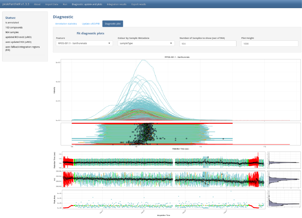
The GUI is to be preferred to understand the methodology, select the best parameters on a subset of the samples before running the command line, or to visually explore results.
If a very high number of samples and features is to be processed,
peakpantheR’s command line functions are more efficient, as
they can be integrated in scripts and the reporting automated.
Input Data
Both real time and parallel compound integration require a common set of information:
- Path(s) to
netCDF/mzMLMS file(s) - An expected region of interest (
RT/m/zwindow) for each compound.
MS files
For demonstration purpose we can annotate a set a set of raw MS spectra (in NetCDF format) provided by the faahKO package. Briefly, this subset of the data from (Saghatelian et al. 2004) invesigate the metabolic consequences of knocking out the fatty acid amide hydrolase (FAAH) gene in mice. The dataset consists of samples from the spinal cords of 6 knock-out and 6 wild-type mice. Each file contains data in centroid mode acquired in positive ion mode form 200-600 m/z and 2500-4500 seconds.
Below we install the faahKO package and locate raw CDF files of interest:
if (!requireNamespace("BiocManager", quietly = TRUE))
    install.packages("BiocManager")

BiocManager::install("faahKO")
library(faahKO)
## file paths
input_spectraPaths  <- c(system.file('cdf/KO/ko15.CDF', package = "faahKO"),
                        system.file('cdf/KO/ko16.CDF', package = "faahKO"),
                        system.file('cdf/KO/ko18.CDF', package = "faahKO"))
input_spectraPaths
#> [1] "C:/R/win-library/4.3/faahKO/cdf/KO/ko15.CDF"
#> [2] "C:/R/win-library/4.3/faahKO/cdf/KO/ko16.CDF"
#> [3] "C:/R/win-library/4.3/faahKO/cdf/KO/ko18.CDF"
Expected regions of interest
Expected regions of interest (targeted features) are specified using the following information:
-
cpdID(character) -
cpdName(character) -
rtMin(sec) -
rtMax(sec) -
rt(sec, optional /NA) -
mzMin(m/z) -
mzMax(m/z) -
mz(m/z, optional /NA)
Below we define 2 features of interest that are present in the faahKO dataset and can be employed in subsequent vignettes:
# targetFeatTable
input_targetFeatTable <- data.frame(matrix(vector(), 2, 8, dimnames=list(c(),
                        c("cpdID", "cpdName", "rtMin", "rt", "rtMax", "mzMin",
                        "mz", "mzMax"))), stringsAsFactors=FALSE)
input_targetFeatTable[1,] <- c("ID-1", "Cpd 1", 3310., 3344.888, 3390., 522.194778,
                                522.2, 522.205222)
input_targetFeatTable[2,] <- c("ID-2", "Cpd 2", 3280., 3385.577, 3440., 496.195038,
                                496.2, 496.204962)
input_targetFeatTable[,c(1,3:8)] <- sapply(input_targetFeatTable[,c(1,3:8)],
                                            as.numeric)
#> Warning in lapply(X = X, FUN = FUN, ...): NAs introduced by coercion| cpdID | cpdName | rtMin | rt | rtMax | mzMin | mz | mzMax |
|---|---|---|---|---|---|---|---|
| NA | Cpd 1 | 3310 | 3344.888 | 3390 | 522.194778 | 522.2 | 522.205222 |
| NA | Cpd 2 | 3280 | 3385.577 | 3440 | 496.195038 | 496.2 | 496.204962 |
Preparing input for the graphical user interface
While the command line functions accept Data.Frame and vectors as
input, the graphical user interface (GUI) will read the same information
from a set of .csv files, or an already set-up
peakPantheRAnnotation object in .RData
format.
We can now generate GUI input files for the faahKO example dataset presented previously:
peakPantheRAnnotation .RData
A peakPantheRAnnotation (previously annotated or not)
can be passed as input in a .RData file. The
peakPantheRAnnotation object must be named
annotationObject:
library(faahKO)

# Define the file paths (3 samples)
input_spectraPaths  <- c(system.file('cdf/KO/ko15.CDF', package = "faahKO"),
                        system.file('cdf/KO/ko16.CDF', package = "faahKO"),
                        system.file('cdf/KO/ko18.CDF', package = "faahKO"))

# Define the targeted features (2 features)
input_targetFeatTable <- data.frame(matrix(vector(), 2, 8, dimnames=list(c(),
                        c("cpdID", "cpdName", "rtMin", "rt", "rtMax", "mzMin",
                        "mz", "mzMax"))), stringsAsFactors=FALSE)
input_targetFeatTable[1,] <- c("ID-1", "Cpd 1", 3310., 3344.888, 3390.,
                                522.194778, 522.2, 522.205222)
input_targetFeatTable[2,] <- c("ID-2", "Cpd 2", 3280., 3385.577, 3440.,
                                496.195038, 496.2, 496.204962)
input_targetFeatTable[,3:8] <- sapply(input_targetFeatTable[,3:8], as.numeric)

# Define some random compound and spectra metadata
# cpdMetadata
input_cpdMetadata     <- data.frame(matrix(data=c('a','b',1,2), nrow=2, ncol=2,
                            dimnames=list(c(), c('testcol1','testcol2')),
                            byrow=FALSE), stringsAsFactors=FALSE)
# spectraMetadata
input_spectraMetadata <- data.frame(matrix(data=c('c','d','e',3,4,5), nrow=3,
                            ncol=2,
                            dimnames=list(c(),c('testcol1','testcol2')),
                            byrow=FALSE), stringsAsFactors=FALSE)

# Initialise a simple peakPantheRAnnotation object
# [3 files, 2 features, no uROI, no FIR]
initAnnotation <- peakPantheRAnnotation(spectraPaths=input_spectraPaths,
                                        targetFeatTable=input_targetFeatTable,
                                        cpdMetadata=input_cpdMetadata,
                                        spectraMetadata=input_spectraMetadata)

# Rename and save the annotation to disk
annotationObject <- initAnnotation
save(annotationObject,
        file = './example_annotation_ppR_UI.RData',
        compress=TRUE)
CSV file input
Another input option for the GUI input consists of a set of
.csv files.
Targeted features
Targeted features are defined in a .csv with as rows
each feature to target (the first row must be the column name), and as
columns the fit parameters to use. At minimum the following parameters
must be defined:
cpdID, cpdName, rtMin,
rt, rtMax, mzMin,
mz, mzMax
If uROI and FIR are to be set, the
following columns must be provided:
cpdID, cpdName, ROI_rt,
ROI_mz, ROI_rtMin, ROI_rtMax,
ROI_mzMin, ROI_mzMax, uROI_rtMin,
uROI_rtMax, uROI_mzMin,
uROI_mzMax, uROI_rt, uROI_mz,
FIR_rtMin, FIR_rtMax, FIR_mzMin,
FIR_mzMax
# Define targeted features without uROI and FIR (2 features)
input_targetFeatTable <- data.frame(matrix(vector(), 2, 8, dimnames=list(c(),
                        c("cpdID", "cpdName", "rtMin", "rt", "rtMax", "mzMin",
                        "mz", "mzMax"))), stringsAsFactors=FALSE)
input_targetFeatTable[1,] <- c("ID-1", "Cpd 1", 3310., 3344.888, 3390.,
                                522.194778, 522.2, 522.205222)
input_targetFeatTable[2,] <- c("ID-2", "Cpd 2", 3280., 3385.577, 3440.,
                                496.195038, 496.2, 496.204962)
input_targetFeatTable[,3:8] <- sapply(input_targetFeatTable[,3:8], as.numeric)

# save to disk
write.csv(input_targetFeatTable,
            file = './1-fitParams_example_UI.csv',
row.names = FALSE)| cpdID | cpdName | rtMin | rt | rtMax | mzMin | mz | mzMax |
|---|---|---|---|---|---|---|---|
| ID-1 | Cpd 1 | 3310 | 3344.888 | 3390 | 522.194778 | 522.2 | 522.205222 |
| ID-2 | Cpd 2 | 3280 | 3385.577 | 3440 | 496.195038 | 496.2 | 496.204962 |
Files to process and spectra metadata (optional)
It is possible to select the files on disk directly through the GUI,
or to select a .csv file containing each file path as well
as spectra metadata. Each row correspond to a different spectra (the
first row must define the column names) while columns correspond to the
path on disk and metadata. At minimum a column filepath
must be present, with subsequent columns defining metadata
properties.
# Define the spectra paths and metada
input_spectraMeta <- data.frame(matrix(vector(), 3, 3,
                        dimnames=list(c(),c("filepath","testcol1","testcol2"))),
                        stringsAsFactors=FALSE)
input_spectraMeta[1,] <- c(system.file('cdf/KO/ko15.CDF', package = "faahKO"),
                            "c", 3)
input_spectraMeta[2,] <- c(system.file('cdf/KO/ko16.CDF', package = "faahKO"),
                            "d", 4)
input_spectraMeta[3,] <- c(system.file('cdf/KO/ko18.CDF', package = "faahKO"),
                            "e", 5)

# save to disk
write.csv(input_spectraMeta,
            file = './2-spectraMetaWPath_example_UI.csv',
row.names = FALSE)| filepath |
|---|
| C:/R/win-library/4.3/faahKO/cdf/KO/ko15.CDF |
| C:/R/win-library/4.3/faahKO/cdf/KO/ko16.CDF |
| C:/R/win-library/4.3/faahKO/cdf/KO/ko18.CDF |
| testcol1 | testcol2 |
|---|---|
| c | 3 |
| d | 4 |
| e | 5 |
Feature meatadata (optional)
It is possible to define some feature metadata, with targeted features as rows (same order as the fitting parameters, first row defining the column names), and as columns the metadata.
# Define the feature metada
input_featMeta <- data.frame(matrix(vector(), 2, 2,
                    dimnames=list(c(),c("testcol1","testcol2"))),
                    stringsAsFactors=FALSE)
input_featMeta[1,] <- c("a", 1)
input_featMeta[2,] <- c("b", 2)

# save to disk
write.csv(input_featMeta,
            file = './3-featMeta_example_UI.csv',
row.names = FALSE)| testcol1 | testcol2 |
|---|---|
| a | 1 |
| b | 2 |
Session Information
#> ─ Session info ───────────────────────────────────────────────────────────────
#>  setting  value
#>  version  R version 4.3.2 (2023-10-31 ucrt)
#>  os       Windows 11 x64 (build 22621)
#>  system   x86_64, mingw32
#>  ui       RTerm
#>  language en
#>  collate  English_United Kingdom.utf8
#>  ctype    English_United Kingdom.utf8
#>  tz       Europe/Paris
#>  date     2023-11-05
#>  pandoc   3.1.1 @ C:/Program Files/RStudio/resources/app/bin/quarto/bin/tools/ (via rmarkdown)
#>
#> ─ Packages ───────────────────────────────────────────────────────────────────
#>  package              * version   date (UTC) lib source
#>  abind                  1.4-5     2016-07-21 [2] CRAN (R 4.3.0)
#>  affy                   1.78.2    2023-07-16 [2] Bioconductor
#>  affyio                 1.70.0    2023-04-25 [2] Bioconductor
#>  Biobase              * 2.60.0    2023-04-25 [2] Bioconductor
#>  BiocGenerics         * 0.46.0    2023-04-25 [2] Bioconductor
#>  BiocManager            1.30.22   2023-08-08 [2] CRAN (R 4.3.2)
#>  BiocParallel         * 1.34.2    2023-05-22 [2] Bioconductor
#>  BiocStyle            * 2.28.1    2023-09-14 [2] Bioconductor
#>  bitops                 1.0-7     2021-04-24 [2] CRAN (R 4.3.0)
#>  bookdown               0.36      2023-10-16 [2] CRAN (R 4.3.2)
#>  bslib                  0.5.1     2023-08-11 [2] CRAN (R 4.3.2)
#>  cachem                 1.0.8     2023-05-01 [2] CRAN (R 4.3.1)
#>  callr                  3.7.3     2022-11-02 [2] CRAN (R 4.3.1)
#>  cli                    3.6.1     2023-03-23 [2] CRAN (R 4.3.1)
#>  clue                   0.3-65    2023-09-23 [2] CRAN (R 4.3.1)
#>  cluster                2.1.4     2022-08-22 [3] CRAN (R 4.3.2)
#>  codetools              0.2-19    2023-02-01 [3] CRAN (R 4.3.2)
#>  colorspace             2.1-0     2023-01-23 [2] CRAN (R 4.3.1)
#>  crayon                 1.5.2     2022-09-29 [2] CRAN (R 4.3.1)
#>  DelayedArray           0.26.7    2023-07-28 [2] Bioconductor
#>  DEoptimR               1.1-3     2023-10-07 [2] CRAN (R 4.3.1)
#>  desc                   1.4.2     2022-09-08 [2] CRAN (R 4.3.1)
#>  devtools               2.4.5     2022-10-11 [2] CRAN (R 4.3.2)
#>  digest                 0.6.33    2023-07-07 [2] CRAN (R 4.3.1)
#>  doParallel             1.0.17    2022-02-07 [2] CRAN (R 4.3.1)
#>  dplyr                  1.1.3     2023-09-03 [2] CRAN (R 4.3.1)
#>  DT                     0.30      2023-10-05 [2] CRAN (R 4.3.1)
#>  ellipsis               0.3.2     2021-04-29 [2] CRAN (R 4.3.1)
#>  evaluate               0.23      2023-11-01 [2] CRAN (R 4.3.2)
#>  faahKO               * 1.40.0    2023-04-27 [2] Bioconductor
#>  fansi                  1.0.5     2023-10-08 [2] CRAN (R 4.3.2)
#>  fastmap                1.1.1     2023-02-24 [2] CRAN (R 4.3.1)
#>  foreach                1.5.2     2022-02-02 [2] CRAN (R 4.3.1)
#>  fs                     1.6.3     2023-07-20 [2] CRAN (R 4.3.1)
#>  generics               0.1.3     2022-07-05 [2] CRAN (R 4.3.1)
#>  GenomeInfoDb           1.36.4    2023-10-02 [2] Bioconductor
#>  GenomeInfoDbData       1.2.10    2023-08-06 [2] Bioconductor
#>  GenomicRanges          1.52.1    2023-10-08 [2] Bioconductor
#>  ggplot2                3.4.4     2023-10-12 [2] CRAN (R 4.3.2)
#>  glue                   1.6.2     2022-02-24 [2] CRAN (R 4.3.1)
#>  gtable                 0.3.4     2023-08-21 [2] CRAN (R 4.3.1)
#>  highr                  0.10      2022-12-22 [2] CRAN (R 4.3.1)
#>  htmltools              0.5.7     2023-11-03 [2] CRAN (R 4.3.2)
#>  htmlwidgets            1.6.2     2023-03-17 [2] CRAN (R 4.3.1)
#>  httpuv                 1.6.12    2023-10-23 [2] CRAN (R 4.3.2)
#>  impute                 1.74.1    2023-05-02 [2] Bioconductor
#>  IRanges                2.34.1    2023-06-22 [2] Bioconductor
#>  iterators              1.0.14    2022-02-05 [2] CRAN (R 4.3.1)
#>  jquerylib              0.1.4     2021-04-26 [2] CRAN (R 4.3.1)
#>  jsonlite               1.8.7     2023-06-29 [2] CRAN (R 4.3.1)
#>  knitr                  1.45      2023-10-30 [2] CRAN (R 4.3.2)
#>  later                  1.3.1     2023-05-02 [2] CRAN (R 4.3.1)
#>  lattice                0.22-5    2023-10-24 [3] CRAN (R 4.3.2)
#>  lifecycle              1.0.3     2022-10-07 [2] CRAN (R 4.3.1)
#>  limma                  3.56.2    2023-06-04 [2] Bioconductor
#>  magrittr               2.0.3     2022-03-30 [2] CRAN (R 4.3.1)
#>  MALDIquant             1.22.1    2023-03-20 [2] CRAN (R 4.3.1)
#>  MASS                   7.3-60    2023-05-04 [3] CRAN (R 4.3.2)
#>  MassSpecWavelet        1.66.0    2023-04-25 [2] Bioconductor
#>  Matrix                 1.6-1.1   2023-09-18 [3] CRAN (R 4.3.2)
#>  MatrixGenerics         1.12.3    2023-07-30 [2] Bioconductor
#>  matrixStats            1.0.0     2023-06-02 [2] CRAN (R 4.3.1)
#>  memoise                2.0.1     2021-11-26 [2] CRAN (R 4.3.1)
#>  mime                   0.12      2021-09-28 [2] CRAN (R 4.3.0)
#>  miniUI                 0.1.1.1   2018-05-18 [2] CRAN (R 4.3.1)
#>  MsCoreUtils            1.12.0    2023-04-25 [2] Bioconductor
#>  MsFeatures             1.8.0     2023-04-25 [2] Bioconductor
#>  MSnbase              * 2.26.0    2023-04-25 [2] Bioconductor
#>  multtest               2.56.0    2023-04-25 [2] Bioconductor
#>  munsell                0.5.0     2018-06-12 [2] CRAN (R 4.3.1)
#>  mzID                   1.38.0    2023-04-25 [2] Bioconductor
#>  mzR                  * 2.34.1    2023-06-19 [2] Bioconductor
#>  ncdf4                  1.21      2023-01-07 [2] CRAN (R 4.3.0)
#>  pander               * 0.6.5     2022-03-18 [2] CRAN (R 4.3.2)
#>  pcaMethods             1.92.0    2023-04-25 [2] Bioconductor
#>  peakPantheR          * 1.16.0    2023-11-04 [1] Bioconductor
#>  pillar                 1.9.0     2023-03-22 [2] CRAN (R 4.3.1)
#>  pkgbuild               1.4.2     2023-06-26 [2] CRAN (R 4.3.1)
#>  pkgconfig              2.0.3     2019-09-22 [2] CRAN (R 4.3.1)
#>  pkgdown                2.0.7     2022-12-14 [2] CRAN (R 4.3.2)
#>  pkgload                1.3.3     2023-09-22 [2] CRAN (R 4.3.1)
#>  plyr                   1.8.9     2023-10-02 [2] CRAN (R 4.3.1)
#>  preprocessCore         1.62.1    2023-05-02 [2] Bioconductor
#>  prettyunits            1.2.0     2023-09-24 [2] CRAN (R 4.3.1)
#>  processx               3.8.2     2023-06-30 [2] CRAN (R 4.3.1)
#>  profvis                0.3.8     2023-05-02 [2] CRAN (R 4.3.1)
#>  promises               1.2.1     2023-08-10 [2] CRAN (R 4.3.1)
#>  ProtGenerics         * 1.32.0    2023-04-25 [2] Bioconductor
#>  ps                     1.7.5     2023-04-18 [2] CRAN (R 4.3.1)
#>  purrr                  1.0.2     2023-08-10 [2] CRAN (R 4.3.1)
#>  R6                     2.5.1     2021-08-19 [2] CRAN (R 4.3.1)
#>  ragg                   1.2.6     2023-10-10 [2] CRAN (R 4.3.2)
#>  RANN                   2.6.1     2019-01-08 [2] CRAN (R 4.3.1)
#>  RColorBrewer           1.1-3     2022-04-03 [2] CRAN (R 4.3.0)
#>  Rcpp                 * 1.0.11    2023-07-06 [2] CRAN (R 4.3.1)
#>  RCurl                  1.98-1.13 2023-11-02 [2] CRAN (R 4.3.2)
#>  remotes                2.4.2.1   2023-07-18 [2] CRAN (R 4.3.1)
#>  rlang                  1.1.2     2023-11-04 [2] CRAN (R 4.3.2)
#>  rmarkdown              2.25      2023-09-18 [2] CRAN (R 4.3.2)
#>  robustbase             0.99-0    2023-06-16 [2] CRAN (R 4.3.1)
#>  rprojroot              2.0.3     2022-04-02 [2] CRAN (R 4.3.1)
#>  rstudioapi             0.15.0    2023-07-07 [2] CRAN (R 4.3.1)
#>  S4Arrays               1.0.6     2023-08-30 [2] Bioconductor
#>  S4Vectors            * 0.38.2    2023-09-22 [2] Bioconductor
#>  sass                   0.4.7     2023-07-15 [2] CRAN (R 4.3.1)
#>  scales                 1.2.1     2022-08-20 [2] CRAN (R 4.3.1)
#>  sessioninfo            1.2.2     2021-12-06 [2] CRAN (R 4.3.1)
#>  shiny                  1.7.5.1   2023-10-14 [2] CRAN (R 4.3.2)
#>  shinycssloaders        1.0.0     2020-07-28 [2] CRAN (R 4.3.2)
#>  stringi                1.7.12    2023-01-11 [2] CRAN (R 4.3.0)
#>  stringr                1.5.0     2022-12-02 [2] CRAN (R 4.3.1)
#>  SummarizedExperiment   1.30.2    2023-06-06 [2] Bioconductor
#>  survival               3.5-7     2023-08-14 [3] CRAN (R 4.3.2)
#>  systemfonts            1.0.5     2023-10-09 [2] CRAN (R 4.3.2)
#>  textshaping            0.3.7     2023-10-09 [2] CRAN (R 4.3.2)
#>  tibble                 3.2.1     2023-03-20 [2] CRAN (R 4.3.1)
#>  tidyselect             1.2.0     2022-10-10 [2] CRAN (R 4.3.1)
#>  urlchecker             1.0.1     2021-11-30 [2] CRAN (R 4.3.1)
#>  usethis                2.2.2     2023-07-06 [2] CRAN (R 4.3.1)
#>  utf8                   1.2.4     2023-10-22 [2] CRAN (R 4.3.2)
#>  vctrs                  0.6.4     2023-10-12 [2] CRAN (R 4.3.2)
#>  vsn                    3.68.0    2023-04-25 [2] Bioconductor
#>  xcms                 * 3.22.0    2023-04-25 [2] Bioconductor
#>  xfun                   0.41      2023-11-01 [2] CRAN (R 4.3.2)
#>  XML                    3.99-0.15 2023-11-02 [2] CRAN (R 4.3.2)
#>  xtable                 1.8-4     2019-04-21 [2] CRAN (R 4.3.1)
#>  XVector                0.40.0    2023-04-25 [2] Bioconductor
#>  yaml                   2.3.7     2023-01-23 [2] CRAN (R 4.3.0)
#>  zlibbioc               1.46.0    2023-04-25 [2] Bioconductor
#>
#>  [1] C:/Temp/RtmpmeNQce/temp_libpath16f061135772
#>  [2] C:/R/win-library/4.3
#>  [3] C:/R/R-4.3.2/library
#>
#> ──────────────────────────────────────────────────────────────────────────────